Categories for Linguistics

Alexis Toumi & Giovanni de Felice

2nd May 2021, Tallcat

1. String diagrams

   • algebraically

   • geometrically

   • combinatorially

2. Formal grammars

   • unrestricted

   • context-free

   • categorial

   • pregroups

3. Functorial semantics

   • Montague semantics

   • recursive neural networks

   • DisCoCat models

We write \(\times\) and \(+\) for the Cartesian product and the disjoint union respectively. For a set \(X\), we write \(X^\star = \coprod_{n \in \mathbb{N}} X^n\) for the free monoid with its unit \(1 \in X^0\) and \(X^\star - \{1\} = \coprod_{n > 0} X^n\) for the free semigroup (i.e. unitless monoid).

String diagrams

Algebraically

Recall:

• A (strict) monoidal category is a category \(C\) together with a functor \(\otimes : C \times C \to C\) that is associative with unit \(1 \in Ob(C)\).

• A functor \(F : C \to D\) is (strong) monoidal when \(F(1) = 1\) and \(F(f \otimes g) = F(f) \otimes F(g)\) for all \(f, g \in C\).

• Thus, we get the category \(\textbf{MonCat}\) of monoidal categories and monoidal functors.

Definition: A monoidal signature is a tuple \(\Sigma = (\Sigma_0, \Sigma_1, \text{dom}, \text{cod})\) where

• \(\Sigma_0\) is a set of generating objects (also called atomic types),

• \(\Sigma_1\) is a set of generating arrows (also called boxes)

• and \(\text{dom}, \text{cod} : \Sigma_1 \to \Sigma_0^\star\) are the domain and codomain.

A morphism of signature \(F : \Sigma \to \Sigma'\) is a pair of functions \(F_i : \Sigma_i \to \Sigma_i'\) for \(i \in \{0, 1\}\) such that \(\text{dom}, \text{cod}(F(f)) = F(\text{dom}, \text{cod}(f))\).

Thus we get the category \(\textbf{MonSig}\) of monoidal signatures and their morphisms.

Let \(U : \textbf{MonCat} \to \textbf{MonSig}\) be the functor which forgets composition and tensor.

Theorem: \(U\) has a left-adjoint \(C_{-}\), where \(C_\Sigma\) is the category of (planar, progressive) string diagrams generated by \(\Sigma\).

References:

• Planar diagrams and tensor algebra, Joyal & Street (1988)

• The geometry of tensor calculus I, Joyal & Street (1991)

• The geometry of tensor calculus II, Joyal & Street (1995)

Geometrically

Definition: A topological graph, also called 1d cell complex, is a tuple \((\Gamma, \Gamma_0, \Gamma_1)\) of

• a Hausdorff space \(\Gamma\),

• a closed, discrete subset \(\Gamma_0 \subseteq \Gamma\) of nodes

• connected components \(\Gamma_1\), called edges, each homeomorphic to an open intervals with boundary in \(\Gamma_0\) such that \(\Gamma - \Gamma_0 = \bigsqcup \Gamma_1\).

Definition: A planar graph between two real numbers \(a < b\) is a finite topological graph \(\Gamma\) embedded in \(\mathbb{R} \times [a, b]\) such that every \(x \in \Gamma \cap (\mathbb{R} \times \{a, b\})\) is a node in \(\Gamma_0\) and belongs to the closure of exactly one edge in \(\Gamma_1\).

The points in \(\Gamma_0 \cap (\mathbb{R} \times \{a, b\})\) are called outer nodes, they are the boundary of the domain and codomain \(\text{dom}(\Gamma), \text{cod}(\Gamma) \in \Gamma_1^\star\) of the planar graph \(\Gamma\).

The points \(f \in \Gamma_0 - (\mathbb{R} \times \{a, b\})\) are called inner nodes, they have a domain and codomain \(\text{dom}(f), \text{cod}(f) \in \Gamma_1^\star\) given by the edges that have \(f\) as boundary.

Definition: A valuation \(v\) of a planar graph \(\Gamma\) in a monoidal category \(C\) is a pair of functions \(v_0 : \Gamma_1 \to \text{Ob}(C)\) and \(v_1 : \Gamma_0 - (\mathbb{R} \times \{a, b\}) \to \text{Ar}(C)\) that send edges to objects and inner nodes to arrows, which respect domain and codomain.

A valued diagram \((\Gamma, v)\) defines a morphism in \(C\), e.g.

\[(B \otimes c \otimes d) \circ (B \otimes B \otimes b \otimes C) \circ (a \otimes B \otimes C)\]

The composition \(\Gamma \circ \Omega\) and tensor \(\Gamma \otimes \Omega\) are defined by rescaling and pasting the two planar graphs \(\Gamma, \Omega\) vertically and horizontally respectively:

Definition: A planar graph \(\Gamma\) is progressive, or recumbent, when the second projection \(e \to [a, b]\) is injective for every edge \(e \in \Gamma_1\). Progressive planar graphs have no cups or caps.

Definition: A progressive planar graph is generic when the projection \(\Gamma_0 - (\mathbb{R} \times \{a, b\}) \to (a, b)\) is injective, i.e. there are no two inner nodes at the same height.

Definition: A deformation of planar graphs is a continuous map \(h : \Gamma \times [0, 1] \to [a, b] \times \mathbb{R}\) such that: * for all \(t \in [0, 1]\), \(h(-, t)\) is an embedding whose image is a planar graph, * for all \(x \in \Gamma_0\), if \(h(x, t)\) is inner for some \(t\) then it is inner for all values of \(t \in [0, 1]\).

A deformation of planar graphs is progressive (generic) when \(h(-, t)\) is progressive (generic) for all \(t \in [0, 1]\).

The induced equivalence relation, i.e. \(\Gamma_0 \sim \Gamma_1\) if and only if there is a deformation \(h\) with \(h(-, 0) = \Gamma_0\) and \(h(-, 1) = \Gamma_1\), is a congruence with respect to composition and tensor of planar graphs.

That is, if \(\Gamma_0 \sim \Gamma_1\) and \(\Omega_0 \sim \Omega_1\) then \(\Gamma_0 \otimes \Omega_0 \sim \Gamma_1 \otimes \Omega_1\) and \(\Gamma_0 \circ \Omega_0 \sim \Gamma_1 \circ \Omega_1\). Furthermore, tensor and composition are associative and they respect the interchange law up to progessive deformation.

Lemma: Progessive planar graphs up to progessive deformation form a strict monoidal category.

Theorem: For a deformation \(h : \Gamma \times [0, 1] \to [a, b] \times \mathbb{R}\) and a valuation \(v\), the value \(v(h(\Gamma, t))\) is indendepent of \(t\).

Theorem: The category of progressive planar graphs valued in \(\Sigma\) (up to progressive deformation) is the free monoidal category \(C_\Sigma\).

Proof: There is a natural isomorphism \(\textbf{MonCat}(C_\Sigma, D) \simeq \textbf{MonSig}(\Sigma, U(D))\).

A functor \(F : C_\Sigma \to D\) is uniquely defined by its image on the signature \(\Sigma\), i.e. by a morphism of signatures. Conversely, a morphism of monoidal signatures \(F : \Sigma \to U(D)\) uniquely extends to a monoidal functor.

Combinatorially

The geometric definition from Joyal & Street is beautiful, but it’s hard to implement as a data structure. We need an equivalent, combinatorial definition.

Reference: * Normalization for planar string diagrams and a quadratic equivalence algorithm, Delpeuch & Vicary (arXiv:1804.07832) * DisCoPy: monoidal categories in Python, De Felice, Toumi & Coecke (arXiv:2005.02975)

Definition: A (strict) premonoidal category is a category \(C\) equipped with a unital, associative functor \(\boxtimes : C \Box C \to C\) where \(C \Box D\) is given by the pushout of the following diagram in \(\mathbf{Cat}\):

\[C_0 \times D \leftarrow C_0 \times D_0 \to C \times D_0\]

where \(C_0, D_0\) are the discrete category of objects and the maps are given by the inclusions.

The pushout \(\Box\) is known as the “funny tensor product”, it may also be defined by the following universal property. Let \(C \Rightarrow D\) be the category with functors \(C \to D\) as objects and the “unnatural transformations” as arrows.

Lemma: \(- \Box C\) is the left adjoint of \(C \Rightarrow -\) in \(\mathbf{Cat}\).

A functor from the funny tensor product \(C \Box D\) can be understood as a functor which is “separately functorial” in its two arguments, in analogy to separate continuity. Premonoidal categories are also known as one-object sesquicategories (one-and-a-half categories) i.e. 2-categories without the interchange law.

Question: Why should we care about premonoidal categories?

Because they actually show up in applications:

• Matrices over a ring form a premonoidal category with the Kronecker product. It is monoidal when the ring is commutative.

• In programming, functions with side effects form a premonoidal categories.

Because they are a middle step towards combinatorial string diagrams:

• They have a simple presentation as free categories.

• Free monoidal categories can then be described as a quotient.

Given a monoidal signature \(\Sigma\), we define a graph \(L(\Sigma)\) with vertices \(\Sigma_0^\star\) and edges \(\Sigma_0^\star \times \Sigma_1 \times \Sigma_0^\star\) with \((u, f, v) : u s v \to u t v\) for \(f : s \to t\). A layer is depicted as a box with wires to its left and right:

We define a diagram \(d\) as a path in the free category generated by the graph of layers \(L(\Sigma)\). It is uniquely defined by:

• a domain \(\text{dom}(d) \in \Sigma_0^\star\),

• a list of \(\text{boxes}(d) \in \Sigma_1^\star\),

• a list of \(\text{offsets}(d) \in \mathbb{N}^{\text{len}(\text{boxes}(d))}\), the number of wires passing to the left of each box.

Two diagrams are equal in the free monoidal category if they are related by a series of interchangers, where \(u, v, w \in \Sigma_0^\star\) and \(s \xrightarrow{f} t, s' \xrightarrow{f'} t' \in \Sigma_1\):

Theorem: The free monoidal category \(C_\Sigma\) is the free category generated by \(L(\Sigma)\), quotiented by the interchangers.

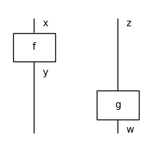
from discopy.monoidal import Ty, Box, Diagram

x, y, z, w = Ty(*"xyzw")
f, g = Box('f', x, y), Box('g', z, w)

assert f @ g == Diagram.decode(
    dom=x @ z,
    boxes_and_offsets=[(f, 0), (g, 1)])

(f @ g).draw(figsize=(2, 2))

from pprint import PrettyPrinter

pprint = PrettyPrinter(sort_dicts=False).pprint
pprint((f @ g).to_tree())

{'factory': 'monoidal.Diagram',
 'inside': [{'factory': 'monoidal.Layer',
             'inside': [{'factory': 'monoidal.Ty', 'inside': []},
                        {'factory': 'monoidal.Box',
                         'name': 'f',
                         'dom': {'factory': 'monoidal.Ty',
                                 'inside': [{'factory': 'cat.Ob',
                                             'name': 'x'}]},
                         'cod': {'factory': 'monoidal.Ty',
                                 'inside': [{'factory': 'cat.Ob',
                                             'name': 'y'}]}},
                        {'factory': 'monoidal.Ty',
                         'inside': [{'factory': 'cat.Ob', 'name': 'z'}]}]},
            {'factory': 'monoidal.Layer',
             'inside': [{'factory': 'monoidal.Ty',
                         'inside': [{'factory': 'cat.Ob', 'name': 'y'}]},
                        {'factory': 'monoidal.Box',
                         'name': 'g',
                         'dom': {'factory': 'monoidal.Ty',
                                 'inside': [{'factory': 'cat.Ob',
                                             'name': 'z'}]},
                         'cod': {'factory': 'monoidal.Ty',
                                 'inside': [{'factory': 'cat.Ob',
                                             'name': 'w'}]}},
                        {'factory': 'monoidal.Ty', 'inside': []}]}],
 'dom': {'factory': 'monoidal.Ty',
         'inside': [{'factory': 'cat.Ob', 'name': 'x'},
                    {'factory': 'cat.Ob', 'name': 'z'}]},
 'cod': {'factory': 'monoidal.Ty',
         'inside': [{'factory': 'cat.Ob', 'name': 'y'},
                    {'factory': 'cat.Ob', 'name': 'w'}]}}

from discopy.drawing import Equation

assert f @ g == f @ z >> y @ g\
             != x @ g >> f @ w\
             == (f @ g).interchange(0, 1)

assert (f @ g).interchange(0, 1).normal_form()\
    == (f @ g).normal_form() == f @ g

Equation(
    (f @ g).interchange(0, 1), (f @ g),
    symbol="$\\mapsto$").draw(figsize=(5, 2))

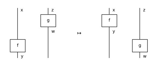
Lemma: Given a boundary-connected diagram with \(n\) boxes, a normal form can be reached in at most \(O(n^3)\) steps.

unit, counit = Box('unit', Ty(), x), Box('counit', x, Ty())
cup, cap = Box('cup', x @ x, Ty()), Box('cap', Ty(), x @ x)

for box in [unit, counit, cup, cap]:
    box.draw_as_spider, box.color = True, "black"

def spiral(n_cups):
    result = unit
    for i in range(n_cups):
        result = result >> x ** i @ cap @ x ** (i + 1)
    result = result >> x ** n_cups @ counit @ x ** n_cups
    for i in range(n_cups):
        result = result >>\
            x ** (n_cups - i - 1) @ cup @ x ** (n_cups - i - 1)
    return result

rewrite_steps = spiral(3).normalize()
Diagram.to_gif(
    *rewrite_steps,
    draw_box_labels=False,
    draw_type_labels=False,
    loop=True, aspect="equal",
    path="../_static/monoidal/spiral.gif")

Input:

• a monoidal signature \(\Sigma\),

• two diagrams \(d, d' \in C_\Sigma\).

Output:

• “Yes” if \(d = d'\),

• “No” otherwise.

Theorem: The word problem for free monoidal categories is solvable in polynomial time.

Formal grammars

Unrestricted

In Probleme über Veränderungen von Zeichenreihen nach gegebenen Regeln (1914), Thue defines what will later be called the word problem for semigroups:

Input:

• a finite set \(X\),

• a finite set of rewrite rules \(R \subseteq (X^\star - \{1\}) \times (X^\star - \{1\})\),

• non-empty sequences \(w, w' \in X^\star - \{1\}\).

Output:

• “Yes” if \(w = w'\) in the semigroup \((X^\star - \{1\}) \sim R\),

• “No” otherwise.

Theorem: The word problem for semigroups is undecidable.

Proof: We can encode the transition table of a Turing machine as a set of rewrite rules, so that solving the Halting problem reduces to deciding equality.

References:

• Recursive Unsolvability of a problem of Thue, Post (1947)

• On certain insoluble problems concerning matrices, Markov (1947)

If we take monoids instead of semigroups, and directed rewrite steps instead of symmetric equality, we can reformulate the problem in terms of free monoidal categories:

Input:

• a monoidal signature \(\Sigma\),

• two types \(w, w' \in \Sigma_0^\star\).

Output:

• a diagram \(d : w \to w'\) in \(C_\Sigma\) if there is one,

• “No” otherwise.

In Syntactic Structures (1957), Chomsky first introduces unrestricted grammars, at the bottom of his well-known hierarchy.

Definition: An unrestricted grammar is a tuple \(G = (V, X, R, s)\) where: * \(V\) is a finite set of terminal symbols (a.k.a the alphabet), * \(X\) is a finite set of nonterminal symbols (a.k.a. grammatical types), * \(R \subseteq \big((V + X)^\star - \{1\}\big) \times (V + X)^\star\) is a finite set of production rules, * \(s \in X\) is the start symbol (a.k.a. sentence type).

The following parsing problem is undecidable:

Input:

• an unrestricted grammar \(G\),

• a sequence \(w \in V^\star\).

Output:

• a diagram \(g : w \to s\) if there is one,

• “Ungrammatical” otherwise.

This motivates the definition of restricted grammars which can still describe the syntax of natural languages but are efficient to parse.

Context-free

Definition: A grammar is context-free when the rules have the shape \(w \to x\) for \(w \in (V + X)^\star\) and \(x \in X\) an atomic type.

Parsings are given by syntax trees with rules as nodes and words as leaves.

Lemma: In a context-free grammar, production rules can be separated in two classes:

• lexical rules of shape \(v \to x\) for a word \(v \in V\) and an atomic type \(x \in X\),

• grammatical rules of shape \(w \to x\) for a sequence of types \(w \in X^\star\) and an atomic type \(x \in X\).

Example:

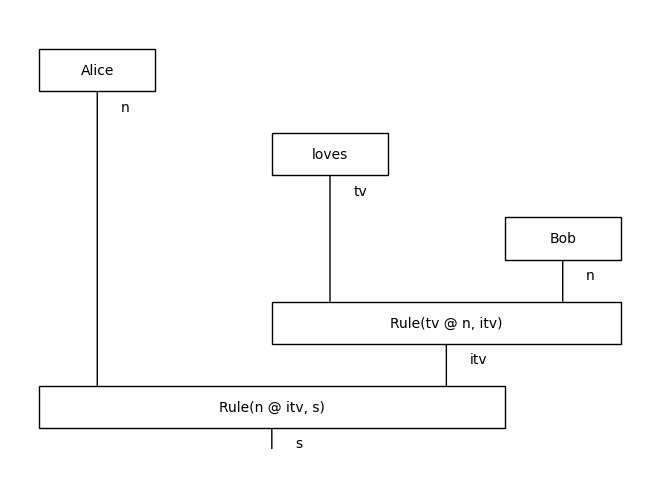
from discopy.grammar.thue import Word, Rule

# sentence, noun, transitive and intransitive verbs
s, n, tv, itv = Ty(*"s n tv itv".split())
words = [Word("Alice", n), Word("loves", tv), Word("Bob", n)]
rules = [Rule(tv @ n, itv), Rule(n @ itv, s)]

tree = Diagram.tensor(*words).foliation() >> n @ rules[0] >> rules[1]

tree.draw()

Theorem: Parsing context-free grammars is \(\mathtt{P}\)-complete.

Categorial grammars

In a categorial grammar, “all the grammar is in the lexicon”.

That is, the only language-dependent rules are the lexical rules, called dictionary entries.

Parsings are given by diagrams in a free biclosed monoidal category.

References:

• Die syntaktische Konnexität, Adjukiewicz (1935)

• A Quasi-Arithmetical Notation for Syntactic Description, Bar-Hillel (1953)

• The Mathematics of Sentence Structure, Lambek (1958)

Definition: A monoidal category \(C\) is left-closed if

• for every pair of objects \(a, b\) there is a hom-object \((a / b)\) and an arrow \(\text{eval}_{a, b} : a \otimes (a / b) \to b\),

• for every arrow \(f : a \otimes c \to b\) there is an arrow \(\text{curry}(f) : c \to (a / b)\) such that \(\text{eval}_{a, b} \circ \text{id}(a) \otimes \text{curry}(f) = f\).

Symmetrically, \(C\) is right-closed if there is a hom-object \((a \setminus b)\).

It is biclosed if it is both left- and right-closed.

Definition: A categorial grammar (a.k.a. AB grammar) is a tuple \(G = (V, X, D, s)\) where:

• \(V\) and \(X\) are finite sets of words and types,

• \(D \subseteq V \times T(X)\) is a finite set of dictionary entries for \(T(X)\) the free \((/, \setminus)\) algebra,

• \(s \in X\) is the sentence type.

A sequence \(w \in V^\star\) is grammatical if there is a diagram \(g : w \to s\) in the free biclosed monoidal category generated by \(D\).

Example:

from discopy.closed import Ty
from discopy.grammar.categorial import Word, BA, FA

s, n = map(Ty, 'sn')

Alice = Word('Alice', n)
loves = Word('loves', (n >> s) << n)
Bob = Word('Bob', n)

sentence = Alice @ loves @ Bob\
    >> n @ FA((n >> s) << n)\
    >> BA(n >> s)

sentence.draw()

Theorem: AB grammars have the same expressive power as context-free grammars.

Pregroup grammars

Half a decade later, Lambek simplified his calculus by going from biclosed to rigid monoidal categories.

References:

• Type grammar revisited, Lambek (1999)

• Type grammars as pregroups, Lambek (2001)

• From word to sentence, Lambek (2008)

Definition: A monoidal category \(C\) is left-rigid (also called left-autonomous) if for every object \(a\), there is a left-adjoint \(a^l\) and a pair of morphisms \(\text{cup} : a^l \otimes a \to 1\) and \(\text{cap} : 1 \to a \otimes a^l\) such that:

\[\text{id}(a) \otimes \text{cup} \circ \text{cap} \otimes \text{id}(a) = \text{id}(a)\]

Symmetrically it right-rigid if every object \(a\) has a right-adjoint \(a^r\).

It is rigid if it is both left- and right-rigid.

from discopy.rigid import Ty, Cup, Cap, Id

x = Ty('x')

left_snake = x @ Cap(x.r, x) >> Cup(x, x.r) @ x
right_snake =  Cap(x, x.l) @ x >> x @ Cup(x.l, x)

assert left_snake.normal_form() == Id(x) == right_snake.normal_form()

Equation(left_snake, Id(x), right_snake).draw(figsize=(5, 2))

Definition: A pregroup grammar is a tuple \(G = (V, X, D, s)\) where:

• \(V\) and \(X\) are finite sets of words and types,

• \(D \subseteq V \times T(X)\) is a finite set of dictionary entries for \(T(X)\) the free \((\otimes, -^l, -^r)\) algebra,

• \(s \in X\) is the sentence type.

A sequence \(w \in V^\star\) is grammatical if there is a diagram \(g : w \to s\) in the free rigid monoidal category generated by \(D\).

Example:

from discopy.grammar.pregroup import Ty, Word, Cup

s, n = Ty('s'), Ty('n')
Alice, Bob = Word('Alice', n), Word('Bob', n)
loves = Word('loves', n.r @ s @ n.l)

sentence = Alice @ loves @ Bob >> Cup(n, n.r) @ s @ Cup(n.l, n)
sentence.draw()

Functorial semantics

Now that we have defined formal grammars as freely generated monoidal categories, we can define natural language semantics as functors!

Montague semantics

Reference:

• English as a formal language, Montague (1970)

• Universal grammar, Montague (1970)

Definition: Montague semantics is a functor \(F : G \to S\) for \(G\) the biclosed category generated by a categorial grammar and \(S\) a free Cartesian-closed category.

Recursive neural networks

Functors from context-free grammars to neural networks.

Reference:

• Parsing Natural Scenes and Natural Language with Recursive Neural Networks, Socher et al. (2011)

DisCoCat

Functors from pregroups to vector spaces.

References:

• A Compositional Distributional Model of Meaning, Clark, Coecke, Sadrzadeh (2008)

• Mathematical foundations for a compositional distributional model of meaning, Clark, Coecke, Sadrzadeh (2010)