hopf

The ribbon category of representations of a finite-dimensional Hopf algebra.

Summary

Algebra	A finite-dimensional Hopf algebra whose structural generators are tensor.Diagrams over one object ty:
Double	The Drinfeld quantum double \(D(H) = H \otimes H^*\) of a Algebra base (Def.
Representation	A finite-dimensional (left) module over the class parameter algebra: given a Algebra H, the class Representation[H] is the type of objects of \(\mathrm{Rep}(H)\), the category Intertwiner[H], and algebra is accessible on both the class and its instances.
Intertwiner	The ribbon category \(\mathrm{Rep}(H)\) of representations of the class parameter algebra: given a Algebra H, the class Intertwiner[H] is a category of tensor.Diagrams whose objects are Representation[H], and algebra is accessible on both the class and its instances.
Functor	A ribbon functor from ribbon diagrams to Intertwiner, i.e. it sends a knot to the tensor network of \(\mathrm{Rep}(H)\) that computes its invariant.

A finite-dimensional quasitriangular Hopf algebra \(H\) has a category of representations \(\mathrm{Rep}(H)\) which is a ribbon category: the braiding is the universal R-matrix, cups and caps come from the antipode, and the twist is the trace of the braid. Both Representation and Intertwiner are class generic over the choice of Hopf algebra: Representation[H] and Intertwiner[H] are the objects and morphisms of \(\mathrm{Rep}(H)\) — a category of tensor.Diagrams whose ribbon structure lives in the classmethods Intertwiner.braid(), Intertwiner.twist(), cups and caps. A quantum topological invariant of tangles is then a ribbon Functor from the free ribbon category into Intertwiner[H], evaluated as concrete tensors (see tensor).

The structural generators of a Algebra (and of a Representation) are stored as tensor.Diagrams, so that composing them, e.g. H.comult >> H.mult, builds a fine-grained network; the network is only contracted (a single einsum) when a morphism is evaluated — by the axiom checks, or by the ribbon Functor on a knot.

Example

The Drinfeld double of the group algebra of \(\mathbb{Z}/2\) gives a non-trivial link invariant: it separates the Hopf link from the two-component unlink.

>>> import numpy as np
>>> from discopy import ribbon
>>> H = Double(Algebra.cyclic(2))
>>> assert H.is_valid() and H.dim == 4
>>> e = Representation[H].anyon(0, -1)
>>> m = Representation[H].anyon(1, 1)
>>> V = Representation[H].direct_sum([e, m])
>>> assert V.is_module()
>>> x = ribbon.Ty('x')
>>> F = Functor(ob_map={x: V}, ar_map={}, cod=Intertwiner[H])
>>> braid = ribbon.Braid(x, x)
>>> hopf_link = (braid >> braid).trace(n=2)
>>> unlink = (ribbon.Cap(x, x.r) >> ribbon.Cup(x, x.r)) @ (
...     ribbon.Cap(x, x.r) >> ribbon.Cup(x, x.r))

The functor gives the tensor network of each knot; contract it with .eval:

>>> hopf = complex(F(hopf_link).eval(dtype=complex))
>>> split = complex(F(unlink).eval(dtype=complex))
>>> assert not np.isclose(hopf, split)
>>> assert np.isclose(hopf, 0) and np.isclose(split, 4)

Because the generators are diagrams, an axiom is an equation of diagrams, checked by contracting both sides (e.g. Algebra.is_associative()). We take a concrete example, the group algebra \(k[\mathbb{Z}/2]\) (generators \(\nabla\), \(\Delta\), …), and both draw and assert each axiom.

>>> from discopy.tensor import Equation
>>> from discopy.tensor import Diagram
>>> H = Algebra.cyclic(2)
>>> ty = H.ty
>>> assert H.is_valid()

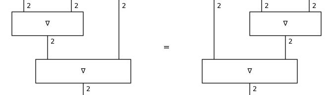
Associativity, (nabla @ H) >> nabla == (H @ nabla) >> nabla:

>>> lhs, rhs = H.mult @ ty >> H.mult, ty @ H.mult >> H.mult
>>> assert H.is_associative()
>>> Equation(lhs, rhs).draw(doctest='docs/_static/hopf/associativity.svg')

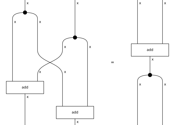
The bialgebra law, Delta is an algebra homomorphism:

>>> lhs = H.mult >> H.comult
>>> rhs = H.comult @ H.comult >> ty @ Diagram.swap(ty, ty) @ ty \
...     >> H.mult @ H.mult
>>> assert H.is_bialgebra()
>>> Equation(lhs, rhs).draw(doctest='docs/_static/hopf/bialgebra.svg')

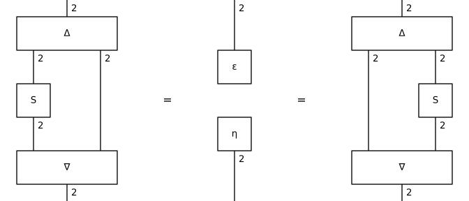
The antipode axiom, comult >> (S @ H) >> mult == counit >> unit:

>>> left = H.comult >> H.antipode @ ty >> H.mult
>>> right = H.comult >> ty @ H.antipode >> H.mult
>>> unit = H.counit >> H.unit
>>> assert H.has_antipode()
>>> Equation(left, unit, right).draw(doctest='docs/_static/hopf/antipode.svg')

The derived generators of the double are composites of the base generators and cups/caps — never materialised. Here is its multiplication, the coadjoint product of \(D(H) = H \otimes H^*\), drawn as a tensor.CMap (the tensor network that gets contracted):

>>> Double(Algebra.cyclic(2)).mult.to_map().draw(
...     doctest='docs/_static/hopf/double_mult.svg')