Diagrammatic Differentiation in Practice

Slides from the Oxford quantum group lunch talk on February 18th 2021.

Implementing automatic differentiation in discopy

from discopy import *
from discopy.quantum import *
from discopy.quantum.zx import Functor, Diagram

from sympy.abc import theta, phi, symbols
from matplotlib import pyplot as plt

Derivatives are compositional: if you have the derivative of each box, then you have the derivative of the diagrams made from those boxes.

x = symbols('x')

f_array = [[1, 0], [0, x]]
g_array = [[1,0,0,0], [0,1,0,0], [0,0,1,0], [0,0,0,x*x]]
h_array = [[1, 1], [1,-1]]

f = QuantumGate('f(x)', n_qubits=1, data=x, array=f_array)
g = QuantumGate('g(x)', n_qubits=2, data=x, array=g_array)
h = QuantumGate('h', n_qubits=1, data=None, array=h_array)

d = {f: [[0, 0], [0, 1]], g: [[0,0,0,0], [0,0,0,0], [0,0,0,0], [0,0,0,2*x]]}

circuit = (f @ h >> g)
circuit.draw(figsize=(3,3))

Given a commutative rig \(\mathbb{S}\), a derivation \(\partial: \mathbb{S} \rightarrow \mathbb{S}\) is defined as any operation that satisfies the linearity and product rules:

\[\partial(f + g) = \partial f + \partial g \quad \text{and} \quad \partial(f \times g) = \partial f \times g + f \times \partial g\]

A related notation is dual numbers \(D[\mathbb{S}]\), numbers of the form \(a + b \epsilon\) for \(a, b \in \mathbb{S}\) such that \(\epsilon^2 = 0\). Sum and product are given by:

Write \(\pi_0, \pi_1 : D[\mathbb{S}] \to \mathbb{S}\) for the projections along the real and epsilon component resp.

Lemma: Every derivation defines a rig homomorphism \(\mathbb{S} \to D[\mathbb{S}]\) with \(f \mapsto f + \partial f\). The other way around, every a rig homomorphism \(\partial : \mathbb{S} \to D[\mathbb{S}]\) with \(\pi_0 \circ \partial = \text{id}_\mathbb{S}\) defines a derivation \(\pi_1 \circ \partial : \mathbb{S} \to \mathbb{S}\).

For example, in the rig of smooth functions we can lift any smooth function \(f : \mathbb{R} \rightarrow \mathbb{R}\) to a function \(f: D[\mathbb{R}] \rightarrow D[\mathbb{R}]\) over the dual numbers defined by:

\[f\left(a+a^{\prime} \epsilon\right)=f(a)+a^{\prime} \times(\partial f)(a) \epsilon\]

Then we can derive the following linearity, product and chain rules:

eps = QuantumGate('eps', n_qubits=0, array=[1e-10])

def DualFunctorAr(box):
    if x in box.free_symbols:
        d_box = QuantumGate(f'd{box.name}', n_qubits=len(box.cod), data=x, array=d[box])
        return box + d_box @ eps
    else:
        return box

dual_functor = CircuitFunctor(ob=lambda x: x,  ar=DualFunctorAr)
test = dual_functor(circuit)
test.draw(figsize=(15, 5))

def project_in_eps(diagram):
    eps_terms = []
    for term in diagram.terms:
        if [box.name for box in term.boxes].count('eps') == 1:
            # remove epsilon
            remove_eps_functor = CircuitFunctor(ob=lambda x: x,
                                                ar=lambda x: Id(0) if x.name == 'eps' else x)
            eps_term = remove_eps_functor(term)
            eps_terms.append(eps_term)
    return Sum(eps_terms, cod=diagram.cod, dom=diagram.dom)

drawing.equation(circuit,
                  project_in_eps(test), figsize=(18, 3), symbol="--dual--> --project-->")

\[\begin{split}\tiny (f(x) \otimes h) \circ g = \left(\begin{pmatrix}1 & 0 \\ 0 & x\end{pmatrix} \otimes \begin{pmatrix}1 & 1 \\ 1 & -1\end{pmatrix}\right) \circ \begin{pmatrix}1&&&\\&1&&\\&&1&\\&&&x^2\end{pmatrix} = \begin{pmatrix}1&1&&\\1&-1&&\\&&x&x^3\\&&x&-x^3\end{pmatrix}\end{split}\]

project_in_eps(test).eval().array.reshape(4, 4)

array([[0, 0, 0, 0],
       [0, 0, 0, 0],
       [0, 0, 1.00000000000000, 3.0*x**2],
       [0, 0, 1.00000000000000, -3.0*x**2]], dtype=object)

Rules for diffentiating diagrams

circuit = (Rx(x) @ Id(1)) >> CX >> (Rx(2*x) @ Id(1))
drawing.equation(circuit, circuit.grad(x, mixed=False), symbol='|--->', figsize=(15, 4))

Rules for differentiating ZX diagrams

XC = QuantumGate('XC', n_qubits=2, array=[[0,1,0,0], [1,0,0,0],[0,0,1,0], [0,0,0,1]])

def gate2zx_new(box):
    from discopy.quantum.zx import gate2zx, PRO, Z, X, Id
    if box == XC:
        return Id(1) @ Z(1, 2) >> X(2, 1) @ Id(1)
    else:
        return gate2zx(box)
circuit2zx = Functor(ob={qubit: PRO(1)}, ar=gate2zx_new, ob_factory=PRO, ar_factory=Diagram)

circuit = (Rx(x) @ Id(1)) >> CX
drawing.equation(circuit, circuit2zx(circuit), circuit2zx(circuit).grad(x), figsize=(9, 2), symbol="---->")

Doubling via the CPM construction

swaps = Id(2) @ SWAP >> Id(1) @ SWAP @ Id(1)
doubled_circuit = swaps[::-1] >> Id(1) @ Rx(-x) @ Rx(x) @ Id(1) >> XC @ CX >> swaps
drawing.equation(doubled_circuit, circuit2zx(doubled_circuit), symbol="--- ZX -->", figsize=(15, 4))

Both Circuits and zx.Diagrams can be differentiated.

doubled_circuit.grad(x, mixed=False).draw(figsize=(12, 4))

circuit2zx(doubled_circuit).grad(x).draw(figsize=(12, 3))

Differentiating a circuit as doubled diagram can give you an asymmetric, undoubled diagram due to the product rule. These diagrams cannot be executed on quantum hardware.

Differntiating Circuits

Similar to how we defined the derivatives of the ZX Spiders in terms of Spiders, the generators of ZX, we need to define the derivatives of the parameterised QuantumGates in terms of QuantumGates

From Schuld et al. the parameter-shift rule for Rz is given by \(\partial R_z(\theta) = \frac{1}{2} [R_z(\theta + \frac{\pi}{2}) - R_z(\theta - \frac{\pi}{2})]\)

drawing.equation(Rz(x).bubble(drawing_name="circ ∂"),
                 Rz(x).grad(x), figsize=(12, 4))

drawing.equation(Rz(x).bubble(drawing_name="double").bubble(drawing_name="diag ∂"),
                 (Rz(-x) @ Rz(x)).grad(x, mixed=False), figsize=(12, 4))

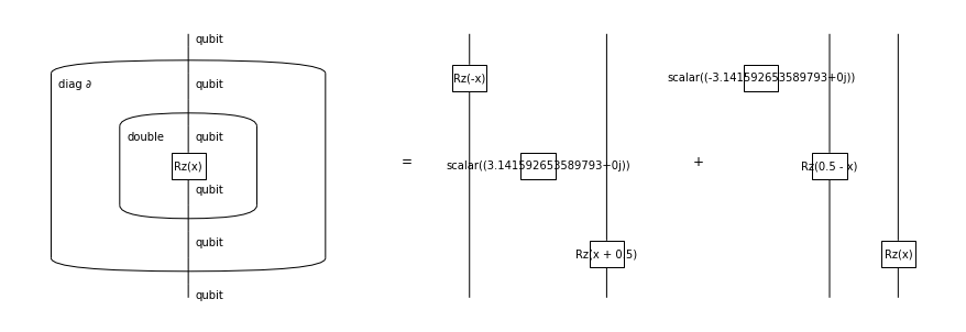
Bear in mind that the previous equation is an equation on circuits, and the this one is an equation on linear maps.

Checks for Diagrams

we checked that the diagrammatic derivatives equals the derivatives of sympy.

import numpy as np
def _to_square_mat(m):
    m = np.asarray(m).flatten()
    return m.reshape(2 * (int(np.sqrt(len(m))), ))

def test_rot_grad():
    from sympy.abc import phi
    import sympy as sy
    for gate in (Rx, Ry, Rz, CU1, CRx, CRz):
        # Compare the grad discopy vs sympy
        op = gate(phi)
        d_op_sym = sy.Matrix(_to_square_mat(op.eval().array)).diff(phi)
        d_op_disco = sy.Matrix(
            _to_square_mat(op.grad(phi, mixed=False).eval().array))
        diff = sy.simplify(d_op_disco - d_op_sym).evalf()
        assert np.isclose(float(diff.norm()), 0.)

test_rot_grad()

Checks for Circuits

we checked that the circuit derivative on the circuit is equal to the diagrammatic derivative of the doubled diagram.

def test_rot_grad_mixed():
    from sympy.abc import symbols
    from sympy import Matrix

    z = symbols('z', real=True)
    random_values = [0., 1., 0.123, 0.321, 1.234]

    for gate in (Rx, Ry, Rz):
        cq_shape = (4, 4)
        v1 = Matrix((gate(z).eval().conjugate() @ gate(z).eval())
                    .array.reshape(*cq_shape)).diff(z)
        v2 = Matrix(gate(z).grad(z).eval(mixed=True).array.reshape(*cq_shape))

        for random_value in random_values:
            v1_sub = v1.subs(z, random_value).evalf()
            v2_sub = v2.subs(z, random_value).evalf()

            difference = (v1_sub - v2_sub).norm()
            assert np.isclose(float(difference), 0.)

test_rot_grad_mixed()

circuit = Ket(0, 0) >> H @ Rx(phi) >> CX >> Bra(0, 1)
gradient = (circuit >> circuit[::-1]).grad(phi, mixed=False)
drawing.equation(circuit, gradient, symbol="|-->", figsize=(15, 4))

x = np.arange(0, 1, 0.05)
y = np.array([circuit.lambdify(phi)(i).eval(mixed=True).array.imag for i in x])
dy = np.array([gradient.lambdify(phi)(i).eval(mixed=False).array.real for i in x])
plt.subplot(2, 1, 1)
plt.plot(x, y)
plt.ylabel("Amplitude")
plt.subplot(2, 1, 2)
plt.plot(x, dy)
plt.ylabel("Gradient")

Text(0, 0.5, 'Gradient')

Bonus: Finding the exponent of a gate using Stone’s theorem

A one-parameter unitary group is a unitary matrix \(U: n \rightarrow n\) in \(\operatorname{Mat}_{\mathrm{R} \rightarrow \mathrm{C}}\) with \(U(0)=\mathrm{id}_{n}\) and \(U(t) U(s)=U(s+t)\) for all \(s, t \in \mathbb{R}\). It is strongly continuous when \(\lim _{t \rightarrow t_{0}} U(t)=U\left(t_{0}\right)\) for all \(t_{0} \in \mathbb{R}\) A one-parameter diagram \(d: x^{\otimes n} \rightarrow x^{\otimes n}\) is said to be a unitary group when its interpretation \([[d]]\) is.

Stone’s Theorem: There is a one-to-one correspondance between strongly continuous one-parameter unitary groups and self-adjoint matrices. The bijection is given explicitly by

\[H \mapsto \exp (i t H)\quad \text{ and } \quad \mapsto-i(\partial U)(0)\]

Future Work

• completing discopy codebase for QML

• solving differential equations

• Keeping derivatives of ZX in ZX, rather than sum of ZX

• Formulate diag diff for Boolean circuits